It saddens me to inform the readers of this blog of the untimely death of Dr. David Ross. David passed away on Saturday, January 14, 2017. David was a great contributor to APICS. He wrote two textbooks that have been used as references in APICS certifications for over a decade.  Seven years ago he joined the APICS staff, originally to recreate the Principles education courses. He designed them to be customizable and companies all around the world are giving their employees targeted training as a result. David created and taught seminars for APICS, presented at our conferences, recorded education presentations and was an essential “in-house’ subject matter expert for the APICS staff. And of course, he wrote these blogs.

David had a huge impact on APICS, our members and customers and the supply chain profession. He will be missed by many, not only for his intellectual achievements, but also for the passion he brought to the subjects he taught, and the people he helped get better at their jobs and careers.

And, so, here is David’s last contribution to the APICS Thinking Supply Chain Blog

Bob Collins, CFPIM, CIRM, CSCP
Senior Director, Professional Development

In the previous blog post, we examined the outcome of three possible sales campaigns. Before progressing, it is important to clarify the sales campaign forecast numbers. In this series of blogs, the sales forecast has been finalized as part of the sales and operations planning (S&OP) process. At this point, the S&OP teams have authorized the demand and supply plans and decomposed the aggregate plans into individual finished goods forecasts. In turn, these values have been loaded into the forecast row of the master schedule.

The below illustration is a representation of the conventional MPS planning grid found in most texts. The grid has been divided into weekly planning periods. The sales campaign timeline has been set at an increment of 8 weeks with a total sales target quantity of 200 units. We are currently in week 5 with the results of the first 4 weeks shown in history. There is a demand time fence (DTF) of 1 week (week 5) detailed in yellow. The planning data appears at the top of the grid. 

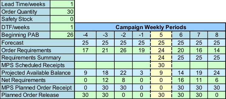
The following observations can be made about the grid results:

1. Sales for the first 4 weeks of the campaign was under plan, totaling 83 units.
2. The end of sales campaign PAB is projected to total 24 units.
3. The first 4 weeks used sold units only as demand, while weeks 6 through 8 used the larger of forecast or actual.
4. An additional total of 99 units (requirements summary) are expected to sell in weeks 5 through 8.
5. In total, by the end of sales campaign period sales is expected to be 182 units, 18 units short of the original forecast for 200.

The next illustration shows the same grid only with higher opening sales.

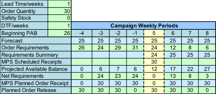
The following observations can be made about the grid results:

1. Sales for the first 4 weeks were over plan, totaling 110 units.
2. The end of sales campaign PAB is projected to total 27 units.
3. An additional total of 99 units (requirements summary) are expected to sell in weeks 5 through 8.
4. In total, by the end of sales campaign period sales is expected to be 209 units, 9 units greater than the original forecast for 200.

Obviously, neither of these results are acceptable. What happens if sales wins a last minute order? What happens if sales in the last weeks goes down instead of up? Is there too much projected inventory at the end of the sales campaign period? In the next blog we will see how converting the MPS to a consumptive forecast built around the sales forecast campaign will solve these problems.